Anna Chambers Portfolio
Description and Motivation:
The motivation of this application is to view the nonemergency 3-1-1 calls over the geographic area of Cincinnati and over the course of 2022 and apply filters to determine trends.
The map portion of the webpage showcases the spread of calls over the Cincinnati area, covering specifically the categories of the calls (ie: Recycling, residential, etc.), agency that responds to the call, and date & response time.
The timeline portion showcases when and what types of calls were placed over the course of 2022 in a monthly and weekly timeframe.
The view below allows you to compare trends across multiple months and categories – the overview is seen in the day timeframe.
The view of word cloud allows you to find the subthemes within the calls that were logged. Due to lag, we only put the first 100 descriptions as proof of concept of the visualization.


Video Demo:
Data:
"This dataset captures All Cincinnati 311 (Non-Emergency) Service Requests from 2012 to present including how long customer service requests have been open, by location, service request type, and department work group. Citizen Service Requests (CSR) give Cincinnati residents the opportunity to submit service request for concerns like potholes, tall grass and missed trash pick-up.
Data Creation: Using the Fix It Cincy! Mobile App, the customer service request online portal and the hotline (513-591-6000), citizen service requests are routed directly to City departments, including Transportation & Engineering, Buildings & Inspections, Health and Public Services. Once the department's work on the service request ticket is completed and the request is marked as "closed," customers receive an email notification that the work has been completed, followed by a link to an optional customer service feedback survey.
Data Created By: The source of this data is the CAGIS."
Note: Only used data from 2022 for our interface. Also only using data with service codes BLD-RES, RCYCLNG, PTHOLE, SIDWLKH, and TIRES to help with load time.
Visualization Components:
In this section, I will show screenshots from the application and explain each view of the data, and each data visualization. I will also go over how to interact with your application, and how the views update in response to interactions.
Map View
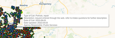
Shown below is the map component of the application. The map shows the location of all of the 311 calls. The user can interact with the map by changing what the calls are colored by and with each color change the legend to the right of the map updates (picture 2). The user can also choose the checkbox to toggle the map between the default street view and an aerial view (picture 3). The map can be brushed to filter by calls only in the brushed area (picture 4). The brushing functionality can be using ctrl + left click while sweeping over the map and this can be discovered by the user by hovering over the information icon (picture 5). The map also shows details about each individual call using tool tips (picture 6).


Timeline View
For the timeline view of the calls, we chose to use bar charts so that the user can clearly see the number of calls associated with the change over time. We divided our timeline into two bar charts, one that shows an overview by months (picture 1) and another that shows a breakdown by days (picture 2). The bar chart by month is used to filter the one by day so that the user can explore different time windows (picture 3). We chose to use selecting of that bar charts to accomplish this instead of brushing so that the user could compare months that are not next to each other (see discoveries section for more details). When the user selects a set of months on the month timeline the day timeline and all other visualizations are filtered by those months (picture 4). The user can also filter down further by selecting a specific day and all other visualizations are updated to just show information from that day (picture 5). Each of the timeline views also shows details (month/day and the number of calls) when you hover over a bar (pictures 6 and 7).


Calls by category Visualization
Our application allows users to learn more about specific details of calls by looking at the calls by category visualization. This visualization is a bar chart that has the x axis updated by a dropdown. This allows the user to explore the number of calls based on service code, agency responsible, response time, day of the week, or zip code. This visualization is filtered by all other visualization selections and also can be used to apply filters by clicking on bars.
Default view

Dropdown options

Graph updated on category change

Filtering chart by other visualizations

Applying new filter
Note: Zip code chart also includes link to map of zipcodes

Tooltip on hover (updated for each category)

Wordcloud Visualization
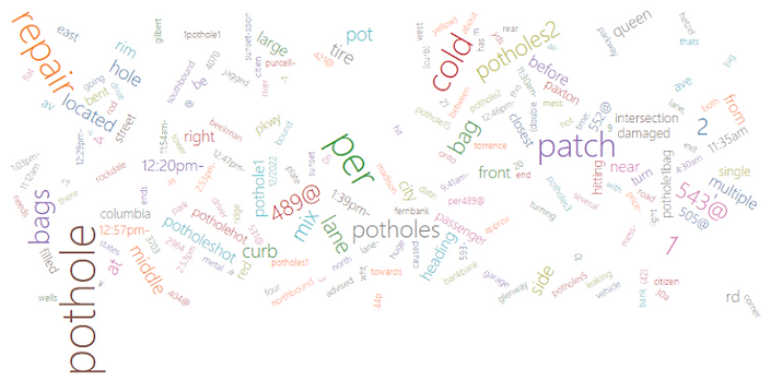
The wordcloud shows all of the important words taken from the unstructured description text of the data. The wordcloud shows the amount of time the word appears by the size of the word (picture 1). This allows the user to determine what is being said in regards to the calls. The wordcloud is updated by the filters applied in all other visualizations (picture 2).

Additionally, since our application can be filtered by many different things at once we included an "Applied Filteres" list that shows all of the filters currently applied ad a "Clear Filters" button to quickly remove all filteres (filters can also be removed one at a time by re-clicking that bar,

Sketches:
Map Sketch
The map is side by side with the color key. Above the map is a dropdown to allow the user to select the color by option. Next to the drop is a check box that will change the map to an aerial view. The key is updated when the dropdown is changed. We will be using a categorial color scale (d3.Category10) because the majority of the color by data type are nominal and we want to keep the color scheme consistent throughout.

Timeline Sketches
Design Challenge technique was used for the timeline sketching. The 5 options purpose was to view the data over different periods of time. After sketching all the possible ideas, the elements and interactive techniques were “selected” for the final views that were implemented in the project.
(Note: sketching was completed before we narrowed down the dataset to just 2022)

This view (interactive bar charts) was selected to be implemented since it makes it easy to break down the different timeframes of the data (Month to day). This also gives the user the flexibility to choose what parts of the timeline to focus on and observe trends. Clicking the specific month (or multiple months) can also combine the analysis of specific times of the year in the timeline with the map visualization.

The tradeoff to using bar charts instead of the line chart was chosen since bar charts show the distribution of calls better over a period of time. The bars allow the user to view the proportions easier than a line chart could provide. IE: If January has 100 calls and March has 5 calls, the proportion is seen more clearly than a line chart.
While we decided to do bar charts instead of a line chart, to consolidate views with the required charts (Service Code, Response Time, Zipcodes, etc.) we decided to use the drop-down to switch between the different relationships.
These 2 views were not used at the end – the interactivity requirement to show multiple periods of time was hard to expand on with a heatmap and scatterplot. Ultimately, the bar charts were the best choice out of the 4 charts to show the number of calls over the month and day timeframe.


Discovery and Findings:
This map visualization allows you to identify trends within specific areas of Cincinnati such as:
-
Most occurring call types by region of Cincinnati
-
Example: Sidewalk and repair hazards occur in counties between Norwalk and Fairfax
-
Example: Residential issues are spread across ALL of Cincinnati
-
-
Agencies that support the community respective to the region of Cincinnati
-
Example: Since the sidewalk and repair is between Norwalk and Fairfax, the Dept of Transportation main area of support is there.
-
-
Response time across the center of Cincinnati is on average 0-9 days
Example: The calls placed over all categories for May and December of 2022. Within May and December, the high and dips are in a similar pattern.

Example: When you click the “Pothole” category in the bar chart, the word cloud updates to only show words from descriptions with the PTHOLE service code (shown below). It can be seen in the lanes have multiple potholes. Glenway is relatively medium in size to show there are a few occurrences in that area.

Example: When filtering by the winter months (December, January, and February), we can see that the most common service called for in Potholes. This would make sense since potholes occur most frequently in the winter due to freezing and thawing of streets.

Process:
Libraries
This project was developed using JavaScript, HTML, CSS, and the d3 library (https://d3js.org/) to help create the visualizations. In addition to d3 we used d3-cloud (https://www.npmjs.com/package/d3-cloud) to help with the development of the wordcloud and leaflet-area-select (https://github.com/w8r/leaflet-area-select) for the functionality of brushing the map.
Code Structure
The code for this application is separated into three main parts: HTML, CSS, and JavaScript files. The HTML file creates the basic structure and layout of the webpage and defines where the visualizations will be placed using svg tags. The CSS file defines the style of the application by indicating the colors and positioning of HTML class values. The JavaScript files contain the main bulk of the logic and create the visualizations. The JavaScript code is organized into classes for each type of chart with one main JavaScript file that initiates, calls, and updates the class objects. We reused one bar chart class for all of the bar charts shown. The main JavaScript file also loads and processes the data and handles filtering.
Access and Run Code
-
Clone the repo or download and unzip
-
In a terminal cd into the downloaded/cloned directory
-
In the same terminal: run `python -m http.server 8000` (for Python 3)
-
Python 2: run `python -m SimpleHTTPServer 8000`
-
Must download Python if not already installed
-
-
Navigate to http://localhost:8000 in a browser
Divison of work:
Anna Chambers: Map Section, Timeline Section (Days), Brushing and Linking Capabilities, Filtering
Keerthi Sekar: Timeline Section (Months), Calls by category bar charts, Wordcloud